


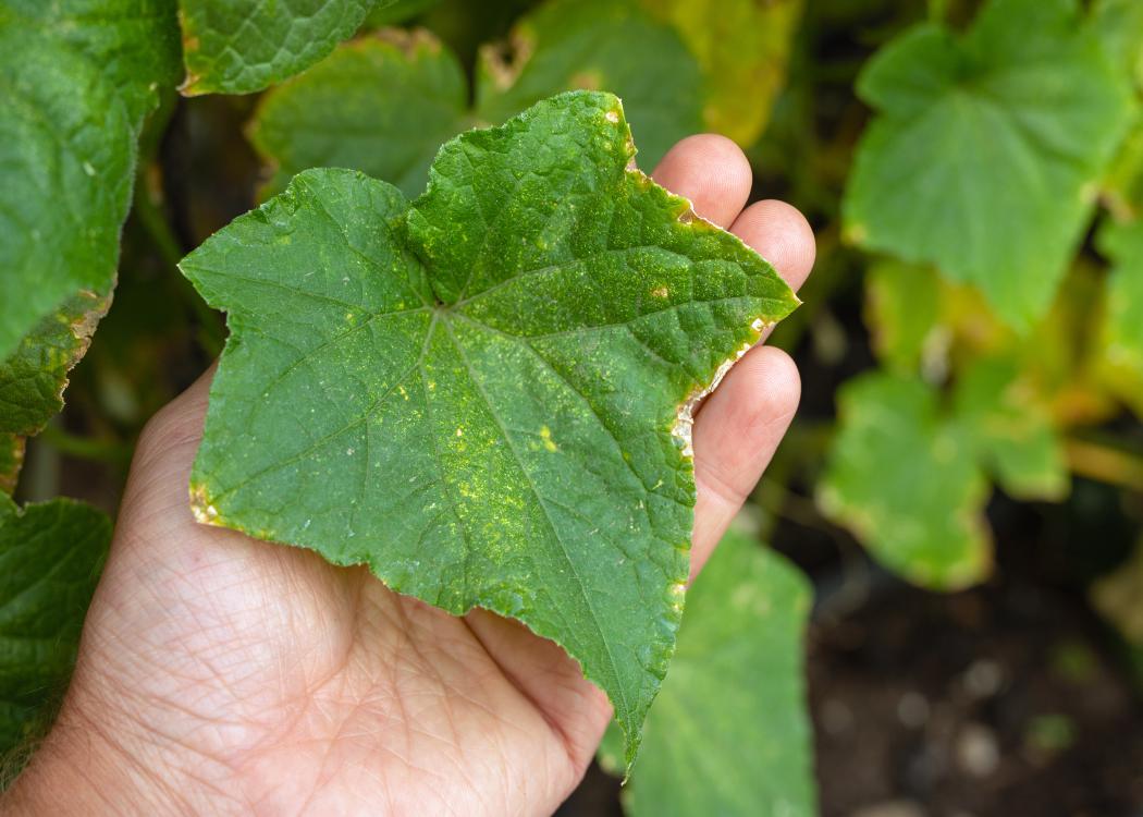
Home vegetable garden plants, like this cucumber plant, are one of the many plants the Mississippi State University Extension Service Plant Diagnostic Laboratory can test for disease. Photo by Olya/stock.adobe.com
Extension for Real Life Blog

")
")
Pages

Select Your County Office
Watch


Extension Matters Magazine
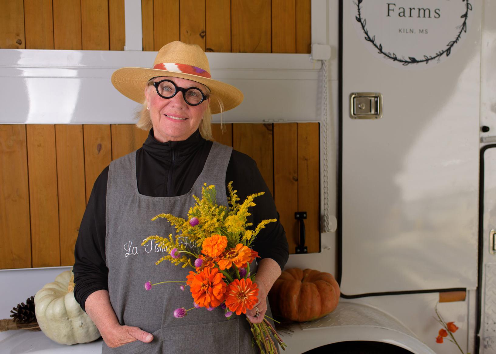
Teri Wyly, co-owner of La Terre Farms in Hancock County
Upcoming Events
Recent Publications
Publication Number: P3201
Publication Number: P3192
Publication Number: P3544
Publication Number: P3551
Publication Number: P3647